Hockey Shot Maps in R: NHL and PWHL Rink Plots with fastRhockey

A shot map puts every shot where it happened on a drawing of the rink. It is the quickest way to see whether a team gets to the slot or settles for the perimeter, and with expected goals (xG) sizing each point, how dangerous those chances were. This article draws NHL and PWHL shot maps, xG shot charts and heatmaps from fastRhockey play-by-play.

What you’ll learn

Which coordinate columns to use for NHL and PWHL shots, and what frame they are in.
How to draw a regulation rink with sportyR and plot shots on it with ggplot2.
How to draw team-coloured rinks with sdvplotR.
How to size shots by xG and build a shot-density heatmap.

You need ggplot2 and sportyR (install.packages(c("ggplot2", "sportyR"))), and optionally sdvplotR (pak::pak("sportsdataverse/sdvplotR")). None of them are fastRhockey dependencies.

library(fastRhockey)
library(dplyr)
library(ggplot2)

# sdvplotR's rinks need sportyR 2.4.5 or later
sdv_ok <- requireNamespace("sdvplotR", quietly = TRUE) &&
  utils::packageVersion("sportyR") >= "2.4.5"

Which coordinates should I use?

Both leagues report locations in feet from centre ice, the frame sportyR draws: x runs along the length of the rink (the goal lines sit at x = ±89 ft), y across it.

League	Columns	Frame
NHL	`x`, `y`	As recorded; teams switch ends each period
NHL	`x_fixed`, `y_fixed`	Intended: home team shooting right. See the caveat below
PWHL	`x_coord`, `y_coord`	As recorded in the HockeyTech feed
PWHL	`x_coord_fixed`, `y_coord_fixed`	Home team shooting right
PWHL	`x_coord_right`, `y_coord_right`	Every team shooting right; `NA` when the event’s side is unknown
PWHL	`x_coord_vertical`, `y_coord_vertical`	Every team shooting up

Coordinate caveats. NHL x_fixed / y_fixed currently ignore the NHL API’s homeTeamDefendingSide: every home-team event is placed at x_fixed >= 0 and every away-team event at x_fixed <= 0. Shots from the attacking zone plot correctly, but shots or other events from a team’s own half are mirrored into its attacking half. A fix is pending; the NHL xG model article shows the effect. For the PWHL, fastRhockey 1.1.0 corrected the derived coordinate columns, and a republish of the PWHL release files with the corrected x_coord columns is pending, so files loaded with load_pwhl_pbp() may predate the fix.

How do I draw an NHL shot map?

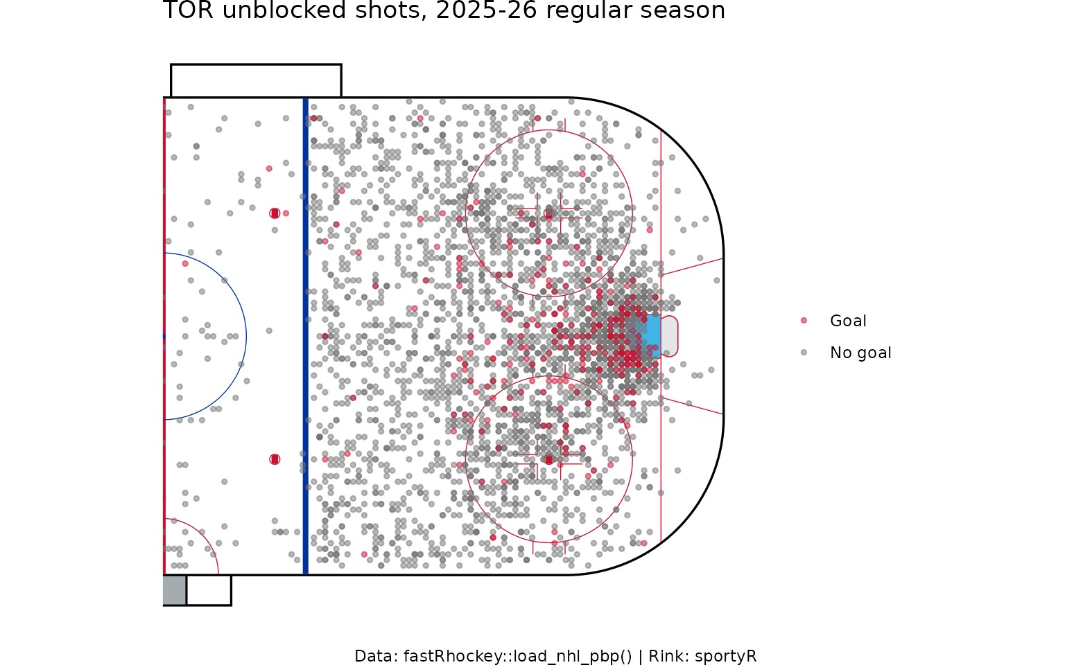
Load a season and keep one team’s unblocked shots. To put every shot in the same attacking end, flip the away team’s coordinates: away events sit at x_fixed <= 0, so negating both coordinates moves them to the right-hand net.

pbp <- load_nhl_pbp(seasons = 2026)

team_abbr <- "TOR"

nhl_shots <- pbp %>%
  filter(
    season_type == "R",
    event_type %in% c("SHOT", "MISSED_SHOT", "GOAL"),
    event_team_abbr == team_abbr,
    !is.na(x_fixed), !is.na(y_fixed)
  ) %>%
  mutate(
    x_plot = if_else(event_team_abbr == home_abbr, x_fixed, -x_fixed),
    y_plot = if_else(event_team_abbr == home_abbr, y_fixed, -y_fixed),
    outcome = if_else(event_type == "GOAL", "Goal", "No goal")
  )

nrow(nhl_shots)
#> [1] 3286

sportyR::geom_hockey() returns a ggplot with the rink already drawn, so you add layers with +. display_range = "offense" shows the right half.

sportyR::geom_hockey("nhl", display_range = "offense") +
  geom_point(
    data = nhl_shots %>% arrange(desc(outcome)),
    aes(x = x_plot, y = y_plot, colour = outcome),
    alpha = 0.5, size = 1
  ) +
  scale_colour_manual(values = c("Goal" = "#C8102E", "No goal" = "grey45"), name = NULL) +
  labs(
    title = paste(team_abbr, "unblocked shots, 2025-26 regular season"),
    caption = "Data: fastRhockey::load_nhl_pbp() | Rink: sportyR"
  )

NHL half-rink shot map of Toronto Maple Leafs unblocked shots in the 2025-26 regular season, goals highlighted.

How do I size shots by expected goals?

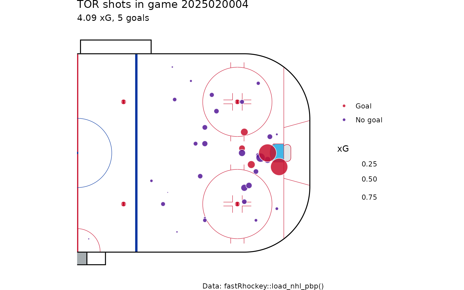
The xg column gives each unblocked shot’s goal probability. Mapping it to point size makes high-danger chances stand out. Here, one game:

one_game <- nhl_shots %>%
  filter(game_id == min(game_id), !is.na(xg))

sportyR::geom_hockey("nhl", display_range = "offense") +
  geom_point(
    data = one_game,
    aes(x = x_plot, y = y_plot, size = xg, fill = outcome),
    shape = 21, colour = "white", alpha = 0.85
  ) +
  scale_size_area(max_size = 10, name = "xG") +
  scale_fill_manual(values = c("Goal" = "#C8102E", "No goal" = "#531896"), name = NULL) +
  labs(
    title = paste(team_abbr, "shots in game", unique(one_game$game_id)),
    subtitle = paste0(round(sum(one_game$xg), 2), " xG, ",
                      sum(one_game$event_type == "GOAL"), " goals"),
    caption = "Data: fastRhockey::load_nhl_pbp()"
  )

NHL half-rink shot map for one game with points sized by expected goals and goals highlighted.

How do I make a shot heatmap?

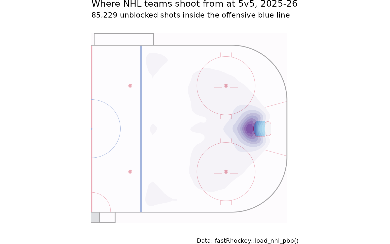
A heatmap shows where shots come from across many games. This one uses every 5v5 unblocked shot in the league, flipped to the same end, with filled density contours.

league_5v5 <- pbp %>%
  filter(
    season_type == "R", strength_state == "5v5",
    event_type %in% c("SHOT", "MISSED_SHOT", "GOAL"),
    !is.na(x_fixed), !is.na(y_fixed)
  ) %>%
  mutate(
    x_plot = if_else(event_team_abbr == home_abbr, x_fixed, -x_fixed),
    y_plot = if_else(event_team_abbr == home_abbr, y_fixed, -y_fixed)
  ) %>%
  filter(x_plot > 25)

sportyR::geom_hockey("nhl", display_range = "offense") +
  stat_density_2d_filled(
    data = league_5v5,
    aes(x = x_plot, y = y_plot),
    alpha = 0.65, bins = 9, contour_var = "ndensity"
  ) +
  scale_fill_brewer(palette = "Purples", guide = "none") +
  labs(
    title = "Where NHL teams shoot from at 5v5, 2025-26",
    subtitle = paste(format(nrow(league_5v5), big.mark = ","), "unblocked shots inside the offensive blue line"),
    caption = "Data: fastRhockey::load_nhl_pbp()"
  )

Filled density heatmap of league-wide NHL 5v5 unblocked shot locations on a half rink, 2025-26.

How do I draw team-coloured rinks with sdvplotR?

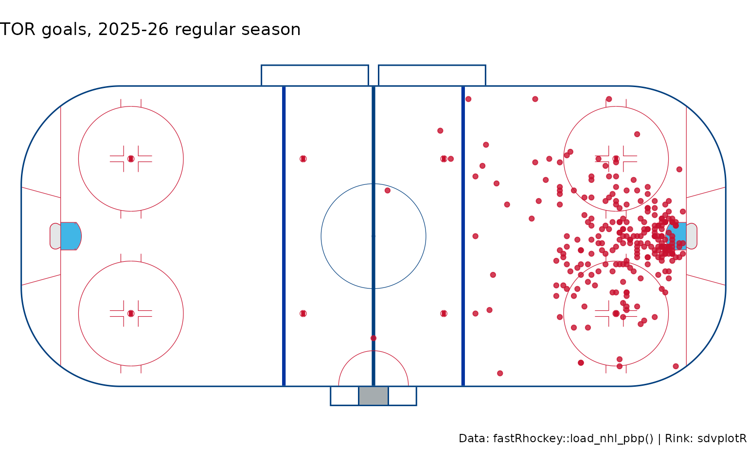
sdvplotR::sdv_surface() draws the same sportyR rinks with SportsDataverse league keys, and with a team it paints the centre line, centre circle and boards in that team’s colours. The league keys for hockey include "nhl", "pwhl", "ahl", "ohl", "whl", "qmjhl", "echl", "ushl", "iihf" and "ncaa_mhockey" / "ncaa_whockey". It needs sportyR 2.4.5 or later; this chunk only runs when that is installed.

sdvplotR::sdv_surface("nhl", team = team_abbr) +
  geom_point(
    data = nhl_shots %>% filter(outcome == "Goal"),
    aes(x = x_plot, y = y_plot),
    colour = "#C8102E", size = 1.5, alpha = 0.8
  ) +
  labs(
    title = paste(team_abbr, "goals, 2025-26 regular season"),
    caption = "Data: fastRhockey::load_nhl_pbp() | Rink: sdvplotR"
  )

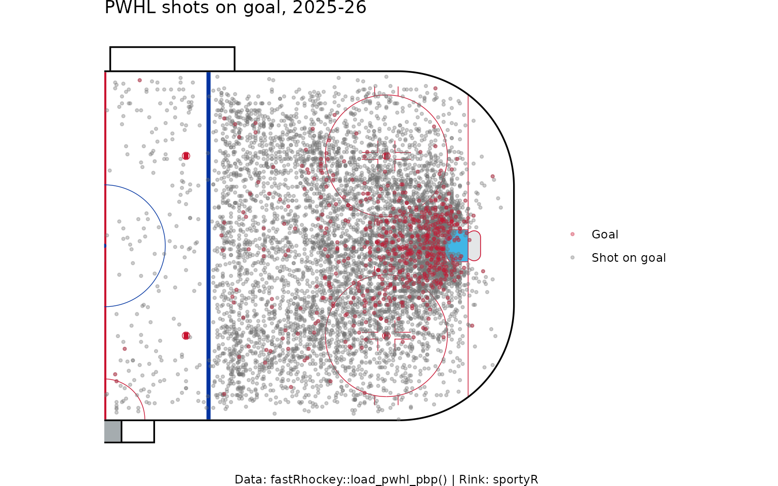
Full NHL rink in Toronto Maple Leafs colours with the team's goals from the 2025-26 regular season.

How do I draw a PWHL shot map?

The PWHL rink in sportyR is geom_hockey("pwhl"). x_coord_right / y_coord_right already put every team shooting right, so no flipping is needed.

pwhl_pbp <- load_pwhl_pbp(seasons = 2026)

pwhl_shots <- pwhl_pbp %>%
  filter(event %in% c("shot", "goal"), !is.na(x_coord_right), !is.na(y_coord_right)) %>%
  mutate(
    team = if_else(team_id == home_team_id, home_team, away_team),
    outcome = if_else(event == "goal", "Goal", "Shot on goal")
  )

count(pwhl_shots, team, sort = TRUE)
#> # A tibble: 8 × 2
#>   team                     n
#>   <chr>                <int>
#> 1 Montréal Victoire     1230
#> 2 Minnesota Frost       1100
#> 3 Ottawa Charge         1066
#> 4 Boston Fleet          1037
#> 5 New York Sirens        947
#> 6 Seattle Torrent        899
#> 7 Toronto Sceptres       899
#> 8 Vancouver Goldeneyes   861

sportyR::geom_hockey("pwhl", display_range = "offense") +
  geom_point(
    data = pwhl_shots %>% arrange(desc(outcome)),
    aes(x = x_coord_right, y = y_coord_right, colour = outcome),
    alpha = 0.35, size = 0.8
  ) +
  scale_colour_manual(values = c("Goal" = "#C8102E", "Shot on goal" = "grey45"), name = NULL) +
  labs(
    title = "PWHL shots on goal, 2025-26",
    caption = "Data: fastRhockey::load_pwhl_pbp() | Rink: sportyR"
  )

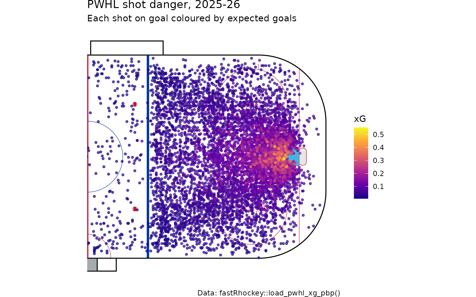
PWHL half-rink map of every shot on goal and goal in the 2025-26 season, goals highlighted.

How do I plot PWHL expected goals?

load_pwhl_xg_pbp() returns one row per shot on goal with an xg column. It carries the feed’s own x_coord / y_coord, where teams attack either end, and no derived columns. You can check against shot_distance: measured to the net at x = +89 ft only about half the shots match, but measured to the nearer net (using abs(x_coord)) they all do.

pwhl_xg <- load_pwhl_xg_pbp(seasons = 2026)

pwhl_xg %>%
  summarise(
    match_net_at_plus_89 = mean(abs(sqrt((89 - x_coord)^2 + y_coord^2) - shot_distance) < 1),
    match_nearer_net     = mean(abs(sqrt((89 - abs(x_coord))^2 + y_coord^2) - shot_distance) < 1)
  )
#> # A tibble: 1 × 2
#>   match_net_at_plus_89 match_nearer_net
#>                  <dbl>            <dbl>
#> 1                0.482                1

So to put every shot in the right-hand end, take abs(x_coord) and flip y_coord for the shots you mirrored.

pwhl_xg_plot <- pwhl_xg %>%
  mutate(x_plot = abs(x_coord), y_plot = if_else(x_coord < 0, -y_coord, y_coord)) %>%
  arrange(xg)

sportyR::geom_hockey("pwhl", display_range = "offense") +
  geom_point(
    data = pwhl_xg_plot,
    aes(x = x_plot, y = y_plot, colour = xg),
    alpha = 0.7, size = 1
  ) +
  scale_colour_viridis_c(option = "plasma", name = "xG") +
  labs(
    title = "PWHL shot danger, 2025-26",
    subtitle = "Each shot on goal coloured by expected goals",
    caption = "Data: fastRhockey::load_pwhl_xg_pbp()"
  )

PWHL half-rink map of shots on goal for 2025-26, coloured by expected goals.

How the PWHL model works is covered in the PWHL expected goals article.

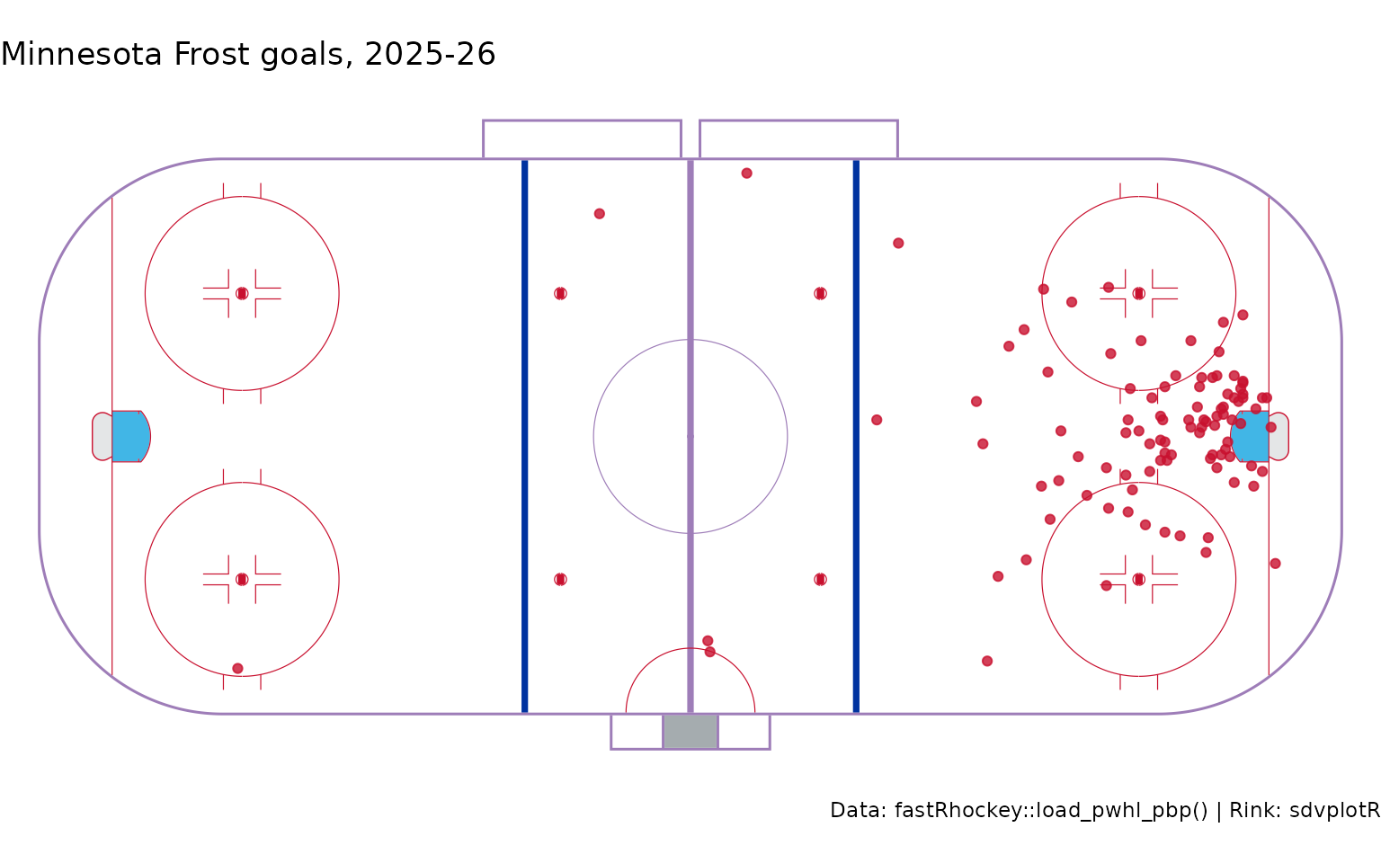
A team-coloured PWHL rink

pwhl_team <- "Minnesota Frost"

sdvplotR::sdv_surface("pwhl", team = pwhl_team) +
  geom_point(
    data = pwhl_shots %>% filter(team == pwhl_team, outcome == "Goal"),
    aes(x = x_coord_right, y = y_coord_right),
    colour = "#C8102E", size = 1.5, alpha = 0.8
  ) +
  labs(
    title = paste(pwhl_team, "goals, 2025-26"),
    caption = "Data: fastRhockey::load_pwhl_pbp() | Rink: sdvplotR"
  )

Full PWHL rink in Minnesota Frost colours with the team's goals from the 2025-26 season.

Other leagues

The AHL, OHL, WHL and QMJHL *_pbp() functions return the same PWHL-style coordinate columns, and sportyR has rinks for "ahl", "ohl", "qmjhl" and more. These are live API calls, so the example is not run here.

ahl_game <- ahl_pbp(game_id = 1000093924)

sportyR::geom_hockey("ahl") +
  geom_point(data = ahl_game, aes(x = x_coord_right, y = y_coord_right))

Several European leagues publish shot locations too (del_shots(), nl_shots(), khl_shots(), liiga_shotmap()); see the European hockey leagues guide. Their coordinate frames differ by provider, so check the ranges before plotting.

Where to go next

NHL expected goals (xG) model and PWHL expected goals (xG) model: what the xG sizes mean.
Corsi, Fenwick and PDO in R: turn shot counts into shot-share metrics.
PWHL and college hockey: more PWHL data.
The sdvplotR NHL shot map recipe for logos and team colours.
Getting started with fastRhockey, and the NHL Data Loaders and PWHL Data Loaders reference sections.

Saiem Gilani, Ben Howell